
A bank approving loans, a telecom flagging churn risk, a hospital predicting readmissions: none of these can ship a prediction alone. Someone has to defend it to a regulator, a loan officer, or a physician. CART was built for exactly that job. It’s a model whose reasoning you can put in front of a human and have them follow it, branch by branch.
Breiman and colleagues introduced CART in 1984, and four decades of faster, more accurate algorithms haven’t displaced it. It handles nonlinear relationships and mixed data types with almost no preprocessing, and it never hides its logic. That combination still runs credit scoring, clinical decision support, fraud detection, and quality control across regulated industries, even where ensembles win on raw accuracy.
What Is CART?
A Classification and Regression Tree (CART) is a supervised learning algorithm that builds a binary decision tree by recursively splitting data into more homogeneous subsets, producing a class label (classification) or a numeric value (regression) at each leaf.
It’s supervised: it learns from labeled historical data and applies those patterns to new cases. The mechanism is recursive partitioning. At each step, the algorithm divides the current data into two groups using whichever feature and threshold produce the most homogeneous split, then repeats on each resulting group. Every internal node has exactly two children, unlike earlier tree algorithms that allow multiway splits.
Breiman, Friedman, Olshen, and Stone formalized this in Classification and Regression Trees (1984), including the impurity measures, pruning method, and surrogate split technique for missing data that later became standard across tree based methods generally.
“CART” covers two related models:
- Classification trees: categorical target (churn / no churn, fraud / legitimate)
- Regression trees: continuous target (price, claim amount)
Both use the same partitioning logic; they differ in how a split’s quality is scored and how leaves generate predictions.
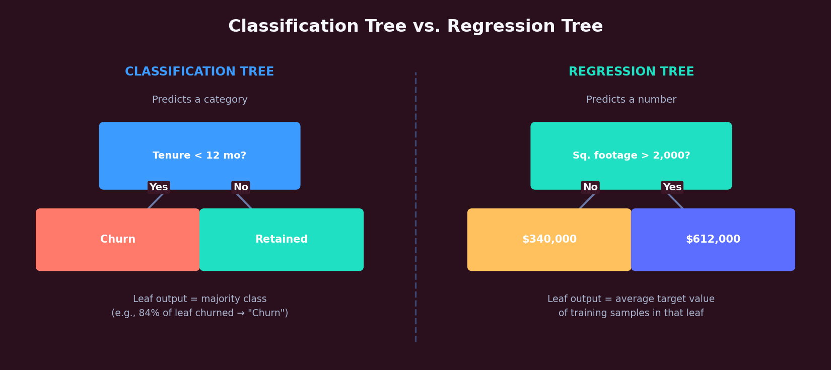
Picture it as an upside down tree. The root asks one question, such as “Is monthly contract value over $70?” Each answer leads to another question, until you reach a leaf with no further questions: the prediction. A customer might flow root, then tenure < 12 months, then support calls > 3, then leaf: “high churn risk.”
How CART Works
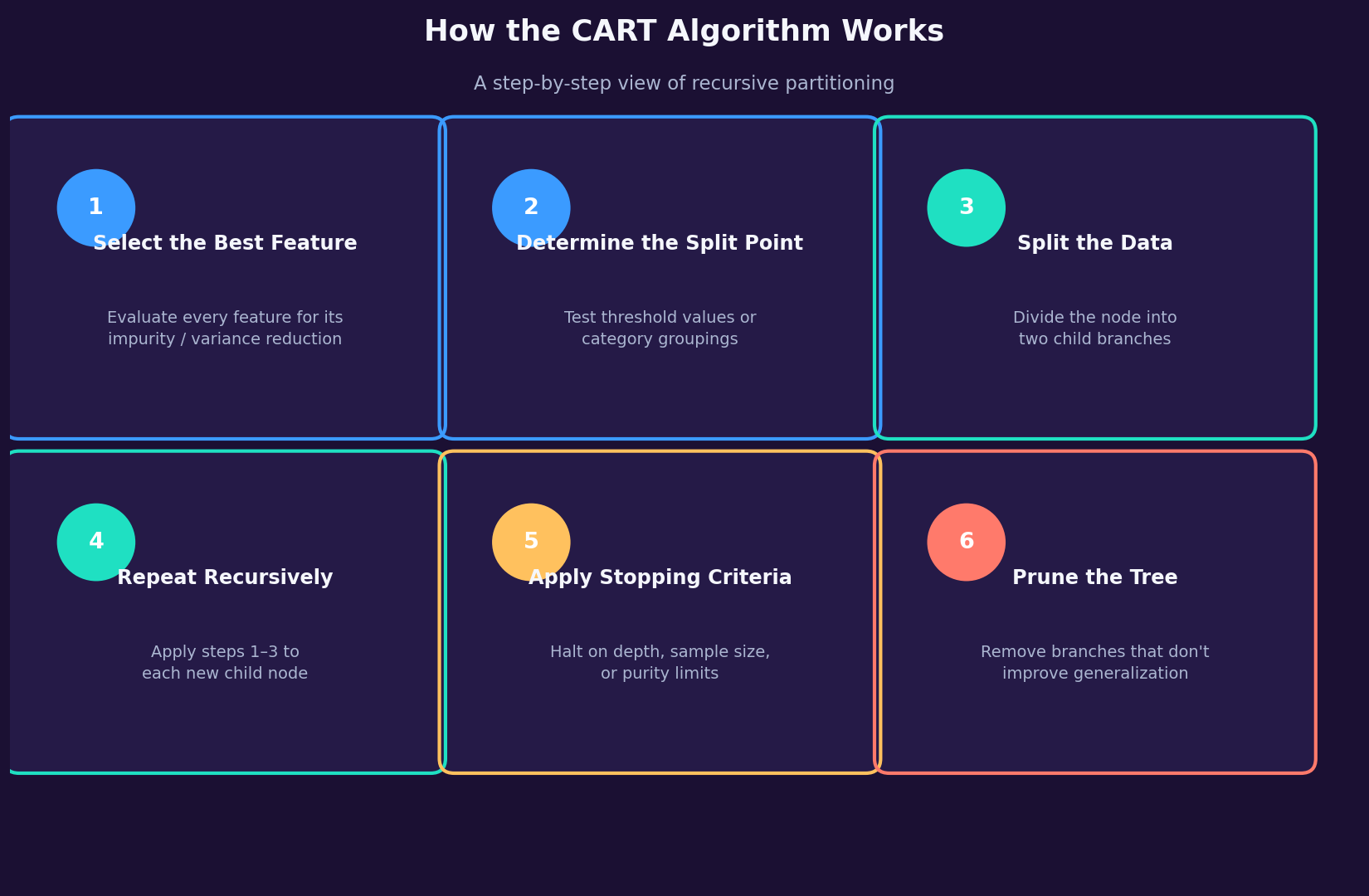
- Select the best feature. Test every feature for how much it would improve purity (classification) or reduce variance (regression) if used to split.
- Find the split point. For that feature, test candidate thresholds or category groupings to find the one with the largest gain.
- Split into two branches.
- Repeat recursively on each child node.
- Stop when a rule is hit: max depth, minimum samples per node, or no further gain.
- Prune the full tree afterward, removing branches that don’t help generalization.
Tree Structure
| Component | Description |
|---|---|
| Root node | The full dataset before any split |
| Decision node | A node that tests a feature and splits into two children |
| Branch | The link between parent and child, representing an outcome |
| Leaf node | A node with no further splits; holds the final prediction |
| Depth | Edges from root to a given node; controls model complexity |
| Split point | The threshold used to divide observations at a node |
Classification vs. Regression Trees
| Attribute | Classification Tree | Regression Tree |
|---|---|---|
| Target | Categorical | Continuous |
| Prediction | Majority class in the leaf | Mean of leaf values |
| Splitting criterion | Gini or entropy | Variance reduction |
| Impurity measure | Gini index, entropy | Sum of squared residuals |
| Evaluation | Accuracy, precision, recall, F1, ROC-AUC | MAE, MSE, RMSE, R² |
| Example use | Will this customer churn? | What will this house sell for? |
Use a classification tree for discrete outcomes (approve/deny, churn/retain). Use a regression tree when the question is “how much.”
Splitting Criteria
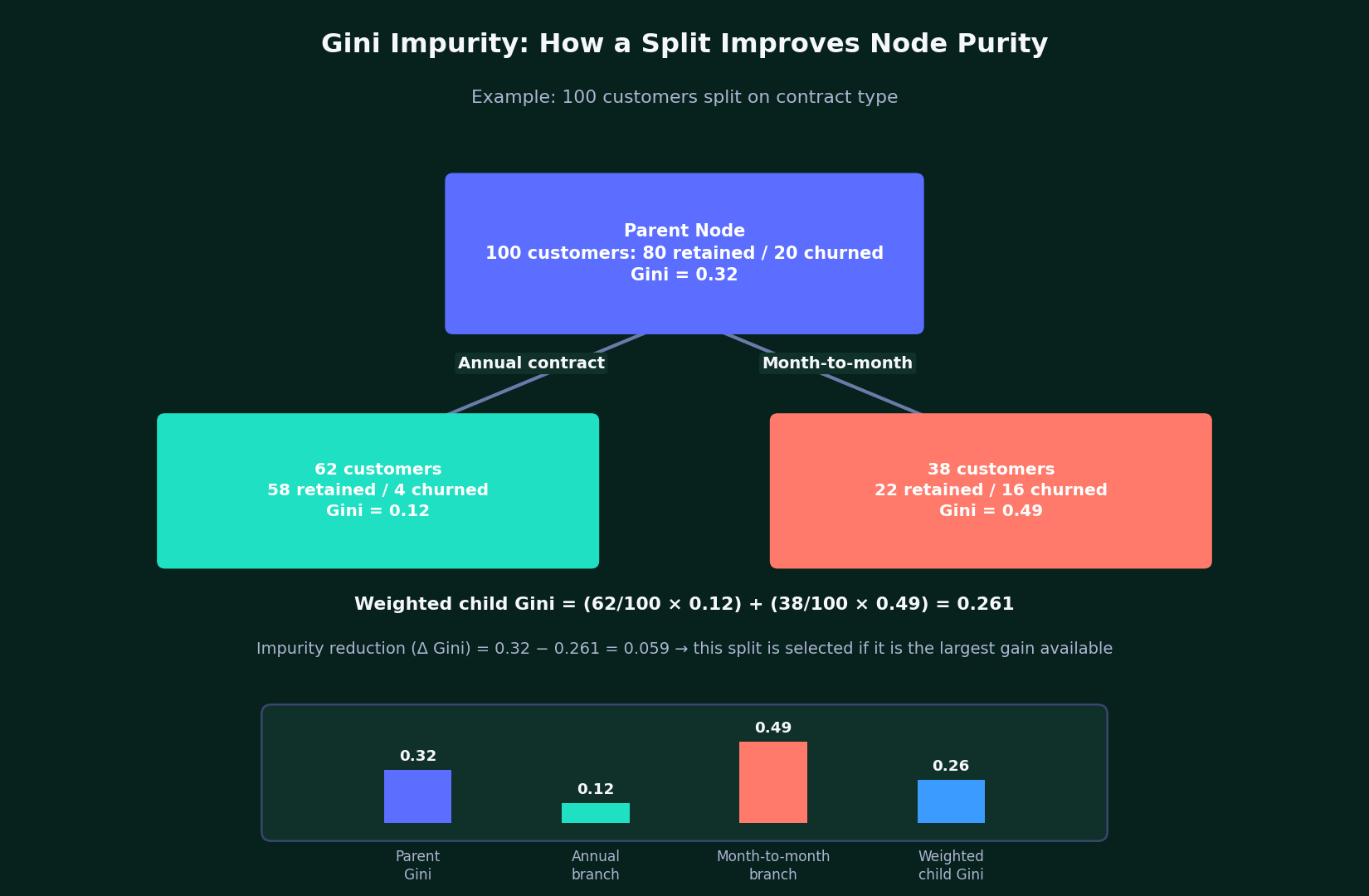
Gini impurity measures how often a random observation in a node would be misclassified if labeled according to the node’s class mix. A pure node scores 0; a 50/50 split scores 0.5 (the maximum for two classes).
Formula: Gini = 1 minus the sum of squared class probabilities.
Example: 100 customers, 80 retained and 20 churned. Gini = 1 − (0.8² + 0.2²) = 1 − 0.68 = 0.32
A candidate split is scored by the weighted average Gini of its two children; the lowest scoring split wins. Scikit-learn defaults to Gini because it’s faster to compute than entropy and usually yields comparable trees.
Entropy, from information theory, measures class unpredictability: 0 for a pure node, 1 at maximum mixing (binary target, log base 2). Same 80/20 example: entropy ≈ 0.72. Information gain is the entropy reduction a split achieves; CART picks the split that maximizes it when entropy is the criterion. Gini and entropy usually produce similar trees; entropy is marginally more expensive and slightly more sensitive to class imbalance.
Variance reduction is what regression trees use instead, since there’s no “class” to measure purity against. A split is scored by how much it lowers combined variance in the two resulting nodes versus the parent. Example: five house prices ($200K, $210K, $205K, $400K, $410K) split on “square footage > 2,500” separates the three smaller homes from the two larger ones, and each group ends up with much lower internal variance than the mixed set.
Formally, at node t, CART searches every feature j and split value s to maximize:
ΔI(s, t) = I(t) − [(n_left/n_t) × I(t_left) + (n_right/n_t) × I(t_right)]
Worked Examples
Churn classification. Features: tenure, monthly charges, contract type, support calls. First split: contract type = month-to-month vs. annual, since month-to-month customers churn far more. Second split, within that branch: tenure < 12 months. A leaf combining month-to-month, under 12 months tenure, and 3+ support calls might hold 90 customers, 76 churned: an implied 84% churn confidence, and a rule a retention team can act on directly.
House price regression. Features: square footage, bedrooms, location, age. First split: square footage > 2,000; second, within the larger home branch: location = urban core vs. suburban. Each leaf reports the average price of training homes that landed there. For example, $612K for large urban-core homes versus $340K for large suburban homes.
Python Implementation
python
import pandas as pd
from sklearn.model_selection import train_test_split
from sklearn.tree import DecisionTreeClassifier, DecisionTreeRegressor, plot_tree
from sklearn.metrics import (
    accuracy_score, precision_score, recall_score, f1_score,
    mean_absolute_error, mean_squared_error, r2_score
)
import matplotlib.pyplot as plt

# Classification
df = pd.read_csv("customer_churn.csv")
X, y = df.drop(columns=["churn"]), df["churn"]
X_train, X_test, y_train, y_test = train_test_split(
    X, y, test_size=0.2, random_state=42, stratify=y
)

clf = DecisionTreeClassifier(
    criterion="gini", max_depth=5,
    min_samples_split=20, min_samples_leaf=10, random_state=42
)
clf.fit(X_train, y_train)
y_pred = clf.predict(X_test)

print("Accuracy:", accuracy_score(y_test, y_pred))
print("Precision:", precision_score(y_test, y_pred))
print("Recall:", recall_score(y_test, y_pred))
print("F1:", f1_score(y_test, y_pred))

plt.figure(figsize=(20, 10))
plot_tree(clf, feature_names=X.columns, class_names=["Retained", "Churned"], filled=True)
plt.show()
python
# Regression
reg_df = pd.read_csv("house_prices.csv")
X_reg, y_reg = reg_df.drop(columns=["price"]), reg_df["price"]
X_train_r, X_test_r, y_train_r, y_test_r = train_test_split(
    X_reg, y_reg, test_size=0.2, random_state=42
)

reg = DecisionTreeRegressor(
    criterion="squared_error", max_depth=6, min_samples_leaf=15, random_state=42
)
reg.fit(X_train_r, y_train_r)
y_pred_r = reg.predict(X_test_r)

print("MAE:", mean_absolute_error(y_test_r, y_pred_r))
print("RMSE:", mean_squared_error(y_test_r, y_pred_r, squared=False))
print("R²:", r2_score(y_test_r, y_pred_r))
Key Hyperparameters
| Parameter | Purpose | Tuning guidance |
|---|---|---|
max_depth | Caps tree levels | Start at 3 to 7 for interpretability; raise while watching validation error |
min_samples_split | Minimum samples to attempt a split | Raise on noisy or small datasets |
min_samples_leaf | Minimum samples per leaf | 10+ smooths predictions, reduces variance |
max_leaf_nodes | Caps total leaves | An alternative complexity control to max_depth |
criterion | Impurity/error function | Gini is faster; entropy is marginally more sensitive to imbalance |
splitter | "best" or "random" | Keep "best" outside randomized ensembles |
random_state | Seeds tie-breaking | Always set for reproducibility |
Tune with cross-validated grid or randomized search across max_depth, min_samples_leaf, and ccp_alpha rather than adjusting parameters one at a time.
Pruning
An unpruned tree tends to overfit: it grows deep enough to memorize noise. Too shallow, and it underfits, missing real patterns. Pruning finds the middle ground.
Pre-pruning constrains growth during training (max_depth, min_samples_split, min_samples_leaf). It’s cheap, but risks stopping before a useful split one level deeper, known as the “horizon effect.”
Post-pruning grows the full tree first, then removes branches that don’t help generalization. It avoids the horizon effect because the whole structure is visible before anything gets cut.
Cost-complexity pruning is CART’s standard post-pruning method:
R_α(T) = R(T) + α × |T|
R(T) is total error, |T| is the number of leaves, and α penalizes complexity. Higher α prunes more aggressively. Scikit-learn’s cost_complexity_pruning_path() returns a sequence of increasing α values, each corresponding to a smaller pruned tree; cross-validation picks the α that minimizes validation error.
python
path = clf.cost_complexity_pruning_path(X_train, y_train)
ccp_alphas = path.ccp_alphas

trees = []
for alpha in ccp_alphas:
    t = DecisionTreeClassifier(random_state=42, ccp_alpha=alpha)
    t.fit(X_train, y_train)
    trees.append(t)

test_scores = [accuracy_score(y_test, t.predict(X_test)) for t in trees]
best_alpha = ccp_alphas[test_scores.index(max(test_scores))]

final_clf = DecisionTreeClassifier(random_state=42, ccp_alpha=best_alpha)
final_clf.fit(X_train, y_train)
The best α usually lands somewhere in the middle of the path: enough pruning to remove noise-driven splits without losing real structure.
Strengths and Limitations
Strengths: fully traceable predictions; handles nonlinear relationships without transformation; mixes numeric and categorical features natively; tolerates missing values via surrogate splits; implicit feature selection (unused features never appear); minimal preprocessing.
Limitations: high variance, meaning a small data change can restructure the whole tree; prone to overfitting without pruning; biased toward features with many distinct values; generally lower accuracy than ensembles like random forests or gradient boosting.
Mitigate with cost-complexity pruning, cross-validation, ensembling when a single tree’s interpretability isn’t required, and care with high-cardinality categorical features.
CART vs. Other Tree Algorithms
| Algorithm | Splits | Criterion | Numeric targets | Missing values | Notable trait |
|---|---|---|---|---|---|
| CART | Binary | Gini / entropy / variance | Yes | Yes (surrogate) | Basis for scikit-learn’s DecisionTree* |
| ID3 | Multiway | Information gain | No | No | Original algorithm; categorical only |
| C4.5 | Multiway | Gain ratio | No | Yes | Adds pruning, continuous features |
| C5.0 | Multiway | Gain ratio (optimized) | No | Yes | Faster commercial successor to C4.5 |
| CHAID | Multiway | Chi-square | No | Yes | Common in market research |
| Conditional Inference Trees | Binary/multiway | Hypothesis testing | Yes | Yes | Reduces bias toward high-cardinality features |
The key distinction: CART always splits into exactly two branches, even for multi-level categorical features, by grouping categories. ID3, C4.5, and CHAID can split into as many branches as a feature has levels, producing shallower trees that are sometimes less stable.
CART vs. Random Forest
| Dimension | CART | Random Forest |
|---|---|---|
| Accuracy | Moderate; overfit-prone | Higher; averaging reduces variance |
| Interpretability | Full tree readable | Hundreds of trees, not individually inspectable |
| Training speed | Fast | Slower |
| Deployment | Lightweight | Heavier, larger and costlier at inference |
| Explainability | Native | Needs tools like SHAP |
| Feature importance | Direct, can be biased | More robust via averaging |
Use CART when a regulator or auditor needs to see the exact decision path, such as adverse-action notices or clinical protocols. Use a random forest when accuracy leads and explainability can be handled post-hoc.
CART vs. Gradient Boosting
Gradient boosting builds trees sequentially, each correcting the last, and typically beats a single CART tree or a forest on tabular accuracy, at the cost of interpretability, training time, and more hyperparameters (learning rate, estimator count, subsampling). Choose standalone CART when the decision path must be individually auditable, when stakeholders need something explainable fast, when the dataset is too small for boosting’s edge to matter, or when regulation calls for a documented, reproducible rule set rather than an ensemble.
Business Applications
- Finance: credit scoring tiers, explainable loan approval, rule-based fraud detection
- Healthcare: disease-risk prediction, patient risk stratification, protocol-style treatment trees clinicians can validate
- Retail: customer segmentation, next-best-offer prediction, stockout/overstock drivers
- Manufacturing: predictive maintenance thresholds, defect-linked process parameters
- Telecom: churn prediction by tenure, usage, and support history; service-quality drivers
- Insurance: claims frequency and severity estimates, transparent underwriting tiers
CART and Explainable AI
CART isn’t an approximation of a more complex model. It is the model, and its logic is readable end to end. That matters for:
- Regulatory compliance: lending and banking rules often require explaining why a specific decision was made for a specific individual; a decision path answers that directly.
- Interpretability: non-technical stakeholders can check the tree against domain expertise.
- Auditability: every split and threshold is explicit and testable against edge cases.
- Documentation: the tree itself is the decision-logic record.
Model Evaluation
Classification: accuracy (misleading on imbalanced data), precision (cost of false positives), recall (cost of false negatives), F1 (balances both), ROC-AUC (ranking ability across thresholds), and the confusion matrix underlying all of them.
Regression: MAE (average absolute error, in original units), MSE (penalizes large errors more), RMSE (MSE back in original units), R² (variance explained, up to 1, can go negative for poor fits).
Best Practices and Common Mistakes
Clean obvious data errors even though CART tolerates missing values and mixed types. Engineer domain-informed features, such as ratios, rolling averages, and recency counts, over raw variables. Hold out a proper test set and use k-fold cross-validation when tuning max_depth, min_samples_leaf, and ccp_alpha. Apply cost-complexity pruning rather than depth limits alone. For imbalanced data, use class_weight="balanced" or resampling instead of relying on accuracy. Watch for leakage: no feature should encode information unavailable at prediction time.
The recurring mistakes: leaving max_depth unset and overfitting; skipping cost-complexity pruning; judging the model on accuracy alone when classes are imbalanced; treating a wildly unstable tree, from a small or noisy dataset, as a red flag to ensemble rather than a modeling choice to defend; deploying without a proper hold-out; and reading high feature importance as proof of causation rather than predictive usefulness.
When to Use CART
- Interpretability is required by regulators, auditors, or non-technical stakeholders
- The relationship between features and target is nonlinear
- Data mixes numeric and categorical types with limited preprocessing time
- The goal includes an explicit, actionable rule set, not just a prediction
- Explainability is a hard requirement, not a nice-to-have
If raw accuracy is the priority and explainability can be handled separately, a random forest or gradient boosting model is usually the better fit, though many teams still start with a CART baseline before layering in something more complex.
Case Study: Cutting Churn With CART
A mid-sized telecom needed to reduce voluntary churn among month-to-month subscribers, and wanted the retention team working from a rule set they could apply without data science support on every campaign.
Data: twelve months of history across roughly 45,000 subscribers, covering tenure, monthly charges, contract type, payment method, support calls, and churn outcome.
Process: an unconstrained tree hit 100% training accuracy but only 71% on test data, a clear overfitting signal. The team ran cost_complexity_pruning_path() and evaluated the resulting trees with 5-fold cross-validation.
Result: the selected tree had 14 leaves and a max depth of 6, deep enough to capture real subsegments and shallow enough to walk through in one meeting. It reached 83% accuracy, 79% recall on the churn class (prioritized since a missed at-risk customer cost more than an unnecessary offer), and a 0.86 ROC-AUC.
Impact: the top three leaves became three targeted retention offers. Illustrative internal tracking over the following two quarters attributed an 18% churn reduction in the targeted segments, roughly $1.2M in retained annual recurring revenue against an $85,000 engagement cost. (Figures are illustrative of a representative engagement, not a specific client’s audited results.)
Need Help Building a CART Model?
An interpretable model is only as good as the pruning, validation, and evaluation behind it. DataScienceConsultingPro.com builds CART models organizations can put in front of regulators and win, from a tree built from scratch to a rescue job on one that’s overfitting in production. That work sits inside our broader machine learning consulting, predictive analytics, and statistical modeling engagements.
FAQ
A supervised algorithm that builds a binary decision tree by recursively splitting data into more homogeneous subsets. Classification trees handle categorical outcomes, regression trees handle continuous ones.
“Decision tree” is the general category; CART is Breiman et al.’s 1984 algorithm within it, distinguished by strictly binary splits, support for both classification and regression, and formalized cost-complexity pruning.
Supervised. It requires labeled historical outcomes to learn from.
A measure of class mixing in a node: the probability of misclassifying a randomly chosen observation given the node’s class distribution. 0 is pure; 0.5 is maximum impurity for two classes.
By routing a new observation to a leaf based on its features, then returning the average target value of the training observations in that leaf.
Removing branches from a fully grown tree that don’t improve generalization, typically via cost-complexity pruning, which weighs error against leaf count.
Yes, by grouping category levels into two subsets at each split, though most implementations, including scikit-learn, require numeric encoding first.
Neither is universally better. CART wins on interpretability and training speed; random forest usually wins on accuracy. Choose based on which one your use case actually needs.
When the relationship is nonlinear, when feature interactions matter more than additive effects, or when the data mixes numeric and categorical features without heavy preprocessing. Linear regression still wins when relationships are genuinely linear and coefficient-level interpretation matters.
DecisionTreeClassifier or DecisionTreeRegressor from scikit-learn: split the data, set hyperparameters like max_depth and min_samples_leaf, fit, predict, and evaluate with the appropriate metrics.
Finance, healthcare, retail, manufacturing, telecom, and insurance: anywhere interpretability matters alongside prediction.
We build, validate, prune, and deploy CART models across the full lifecycle, from dataset assessment and feature engineering through optimization and production deployment, with an emphasis on interpretable, auditable results.
